Home Browse Search & Custom Hierarchy Download Errors About Links

Outline

Most proteins act in concert with other proteins, forming permanent or transient complexes. Understanding these interactions at an atomic level is only possible through analysis of protein structures. Over the past few years, there have been efforts to infer the quaternary structures of X-ray crystal structures (Henrick and Thornton 1998; Valdar and Thornton 2001; Ponstingl, Kabir et al. 2003; Bahadur, Chakrabarti et al. 2004), which support the prediction of the Biological Unit to the structure in PDB.

Based on these predictions, we present a visualization and comparison strategy, and construct a hierarchical classification of complexes to integrate and organise the structures. Our strategy is organized in two main steps that we illustrate below:

1. The representation of proteins complexes as graphs,
2. The comparison of the graphs.

We also discuss about the symmetry types that are found in protein complexes, and brief explanations can be found here

Main steps involved in building 3D Complex

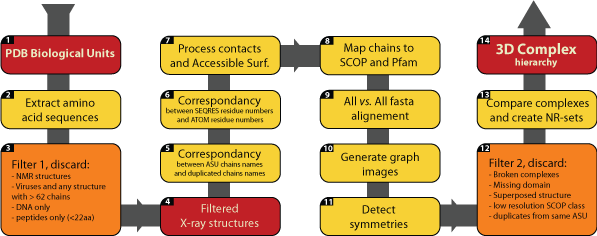
Flowchart highlighting the main steps involved in builing 3D Complex. The steps 10, 13 and 14, which are critical are discussed in more detail below

1. All the PDB Biological Units are downloaded from the EBI web-site,
2. Both the amino-acid sequences from the SEQRES and ATOM fields are extracted. All informations relative to the structure (e.g. Title, Resolution etc.) are also extracted,
3. We discard all NMR structures, as well as those that do not contain a protein or those that are too large,
4. At this stage we have a dataset of X-ray structures which are further processed,
5. Sometimes chains are duplicated to create a Biological Unit (see below), therefore we rename duplicated chains and keep track of the correspondancies.
6. Sometimes, even in the remediated PDB, the residue numbers in the ATOM field are wrong. To correct this, we align the ATOM sequences on the SEQRES sequences and renumber them accordingly.
7. We then process contacts between the chains.
8. In order to detect homology relationships, we calculate the N- to C- terminal domain architecture of each chain according to SCOP and Pfam.
9. We then precompute an all VS. all fasta sequence alignment. This is used to infer which complexes are homo-oligomers, and is also used in PiQSi for browsing homologs in the PDB. There are ~38,000,000 million hits!
10. At that point, for any complex we know (i) which chains are in contact (step 7), (ii) which chains are identical (step 9), (iii) which chains are homologous (step 8). We use this information to generate a 2D graph cartoon for each complex as detailed below.
11. We then search for internal point symmetries within each complex, as detailed in the primary reference. we use this information as an indicator of the spatial 3D structure, in particular for homo-oligomers.
12. At this point, we remove a number of problematic structures. Broken complexes are structures split in two or more sub-complexes when 'removing' subunit-subunit contact containing less than five amino-acids; 'Missing domains' are structures with no information on domain architecture in SCOP; Superposed structures are artifacts where two chains are completely superposed; low resolution structures often contain C-alphas only and thus cannot be used for calculating subunit-subunit contacts; finaly when the ASU contains 2 or more Biological Units, several PDB identifiers exist (e.g. 1k8c_1, 1k8c_2), where '_1' is the number of the Biological Unit. Thus, we keep one copy per only per PDB code. When the copies are different from each others, we choose one by hand.
13. This gives us the final dataset of monomers and complexes, that we compare using their graphs representation and a graph-matching algorithm.
14. We then assemble the non-redundant datasets so obtained in order to create the final 3D Complex Hierarchy

Representing Protein Complexes as Graphs

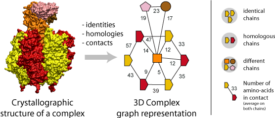
A fundamental step of our method is the translation of each protein complex into a graph. This involves processing the identities, homologies and contacts between the chains within each complex. Structural homology is detected using the N- to C-terminal order of SCOP superfamilies also called the domain architecture, and sequence identity is detected after a FASTA alignment with a 99% sequence identity threshold. Protein-protein interfaces are defined by a threshold of at least ten residues in contact, where the number of residues is the sum contributed by both chains. A residue-residue contact is counted if any pair of atomic groups is closer than the sum of their Van der Waals radii plus 0.5 � (Tsai, Taylor et al. 1999).

The graph itself thus provides the topology of the complex, i.e., the number polypeptides chains (nodes) together with their pattern of interfaces (edges), and an additional label associated to each graph carries the complex symmetry. Also, a label on each edge indicates the number of residues at the interface.

Importantly, the color and shapes of nodes are consistent within a graph but not among different graphs

Comparing Protein Complexes to construct a hierarchy

Once we have translated all protein complexes into their corresponding graph, we compare them with each other in order to build the hierarchy. From the graph representation, we have access to four types of information about each complex:

1. The topology, represented by the number of nodes and their pattern of contacts,
2. The structure of each constituent chain in the form of SCOP domain architecture,
3. The amino acid sequence of each constituent chain, and thus the number of identical and homologous chains,
4. The symmetry of the complex.

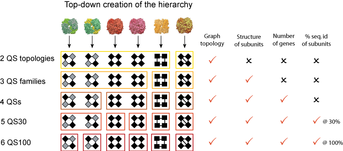
With these four types of information, we elaborate progressively stricter criteria that we use for comparing and grouping complexes, as illustrated in the figure above. First we group complexes according to their topology (e.g. their number of chains + pattern of contacts). Each of these groups is a QS Topology.

We then break down QS topologies into smaller groups called QS Families. In these, complexes have chains that are similar to each other structurally (e.g. same SCOP domain architecture). This means that two complexes in the same QS Family can be distantly homologous, sharing structural similarity but very little sequence identity. At the next level, we include the requirement that two matching complexes must have an identical number of genes. This is illustrated with hemoglobins in the figure above, where the hemoglobin α2β2 and the hemoglobin γ4 are in the same QS Family but in different QSs

From level four onwards, we require sequence homology between two matching chains, from 20% identity (4th level) to 100% (12th level). We call these groups QS20/30/40 etc. As the sequence similarity threshold gets stricter, the Quaternary Structure groups break down into smaller sub-groups.

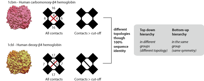
In top-down hierarchy, complexes with different topologies are never grouped together. This can be problematic in respect of the redundancy because closely related complexes can have different topologies, as illustrated with two human hemoglobin β4 homotetramers above. Therefore, in addition to the top-down hierarchy we provide a bottom-up hierarchy, where these two complexes are grouped together. The bottom-up hierarchy is identical to the top-down, except for homo-oligomers, which are grouped together on the basis of their symmetry instead of their topology. If you intend to carry out an analysis on homomers, we recommend the use of the bottom-up hierarchy.

The PDB Biological Unit

X-ray crystallography is the most common method used to gain information about protein structure. Structures obtained with this method correspond to an asymmetric-unit (ASU) i.e. the minimal unit from which the whole crystal can be reconstructed using symmetry operations. Importantly, the protein(s) contained in the ASU may not be in their native functional oligomeric state. For example, an ASU may contain a single copy of a protein that actually forms a homohexamer in vivo, or it might contain a dimer of a protein that exists as a monomer in vivo. This is why, in addition to the coordinates of the ASU, the Protein Data Bank makes available the coordinates of the Biological Unit, which is believed to contain the structure of the protein in its native state. For structures released up to 1998, the Biological Units are created automatically using the Protein Quaternary Structure server (PQS, (Henrick and Thornton 1998)). For structures from 1998 onwards, which are the majority of structures in PDB, the Biological Unit is manually curated and inferred based on the expertise of the authors of the structure as well as the PDB curators.

Symmetry of homomers

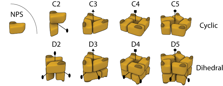
Homomers are very abundant in nature and also in 3D Complex, where they account for 90% of the complexes. They can be separated into two main classes of open or closed symmetry. The first class corresponds to open structures that would polymerize to infinity in the absence of limiting factors (not shown here). Such assemblies (e.g. tubulin and actin) are rare in 3D Complex (3%), most likely due to their innate dynamic character rendering them difficult to crystallize. By contrast closed symmetries are finite in space, and most homomers adopt either cyclic or dihedral symmetry (shown in Figure), with only a small fraction (1%) with cubic symmetry like virus' capsids (not shown). In 3D Complex we denote Cn a cyclic complex containing n subunits, and Dn as a dihedral complex containing 2*n subunits. In the figure, dotted lines with elipses, triangles, square and pentagons represent 2-, 3-, 4-, and 5- fold symmetry axes respectively.